This post is a continuation of the first part about my Voronoi Shattering project, please make sure to read it first.
Fragment carving
On the previous post we left it at the point where we had a Voronoi Diagram generated from a set of points sampled from the source geometry’s volume. We’ll now take it from there and, in this post, I’ll be talking about the mesh slicing.
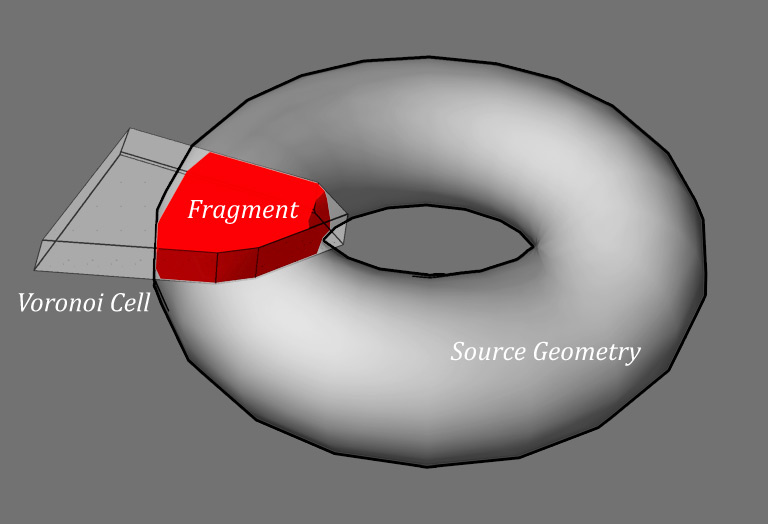
Fig. 1. Voronoi cell intersecting source geometry to form fragment
Given the voronoi diagram and the input geometry, the way to obtain the fragments for our shatter algorithm is by computing the intersection of the mesh with each one of the voronoi cells (Fig 1). Since the VD define a convex hull, it means that we can calculate the intersection with the simple following method:
For each voronoi cell C do For each face F in C do Obtain the plane P containing F Split the geometry in two using P, and discard all the polygons on the front side of P Identify the set of vertices lying exactly on P, and generate a new set of faces filling the hole. end end 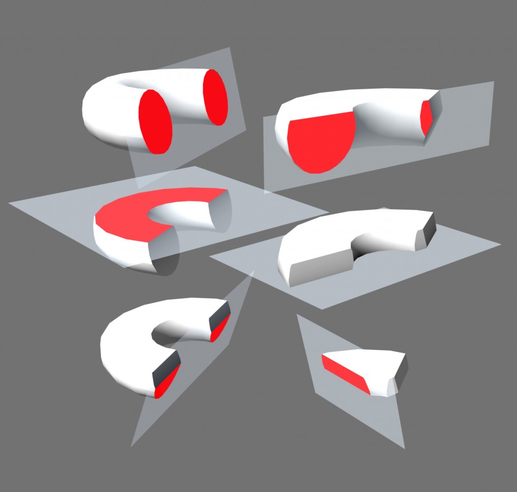
Fig 2. Slicing the geometry with the faces of a VD cell
The process is depicted in Fig. 2. Note that by filling the holes left from each cut before we move on to the next one -marked as red faces in the picture-, we solve the problem of keeping the shape closed defining a volume.
Hole filling
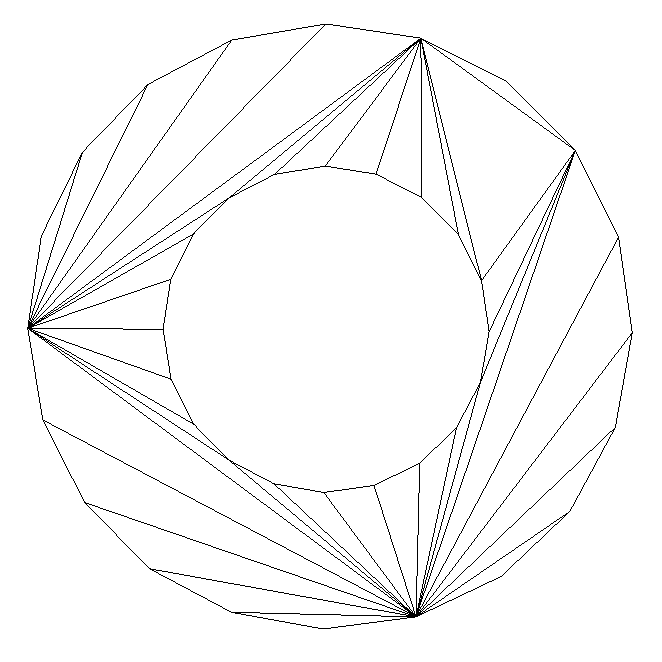
Fig. 3. First attempt – Naive tessellation
Filling the holes left by each cut while we’re carving the shape is a matter of triangulating a flat set of vertices lying exactly over the cut plane. The vertices will be a combination of new vertices generated by splitting existing faces, and a few more previously existing ones, which happened to be coplanar already. Linking the vertices we’ll have edges describing outlines and holes (e.g. when we slice a torus in two as in Figure 3), and since everything happens on a plane we can just project the coordinates from 3D to 2D, triangulate, and then reproject the result back to 3D.
I initially made the mistake of going for a overly simplistic approach that led to more problems than actual benefits – I’m describing it here anyway possibly as an example of something that didn’t go well!
Version 1 of my hole filling algorithm was trying to identify sequences of linked segments describing loops. Then the relative position of those loops was tested to determine which of them were outlines and which were holes. Next, for every set of outline and its contained holes, every pair of vertices was linked with a new edge unless that edge would intersect with an existing one. The result is depicted in Figure 3.
Unfortunatelly there were several problems with this approach:
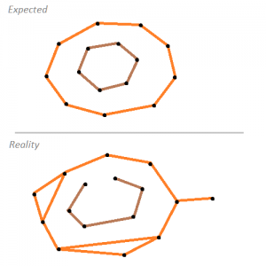
- First of all, identifying the closed loops from a pool of edges turned out to be harder than expected: ideally it would be a matter of finding a sequence of edges v1-v2, v2-v3, v3-v4… eventually finding edge vn-v1 closing the loop. However, tiny imperfections on the mesh slicing such as parallel faces perpendicular to the plane or just tiny or degenerated faces being discarded would cause missing edges -open loops-, inner loops or dangling segments, and an overall actual input being far from the ideal expected, see Figure 4.
- Missing edges were particularly harmful because they would cause loop sequences not to be found, this then resulting in entire holes not being filled. When the shape (now left open) was sliced again, even more edges would be missing, just making things worse and worse.
- Even when things didn’t go wrong, the quality of the triangulation was not very good, being very prone to stretched triangles that would just cause further trouble when being sliced.
The overall method, despite being simple in principle, turned out to be not so simple in practice when having to deal with real-world details, and above all, it happened to be just too fragile for it to work for the general case.
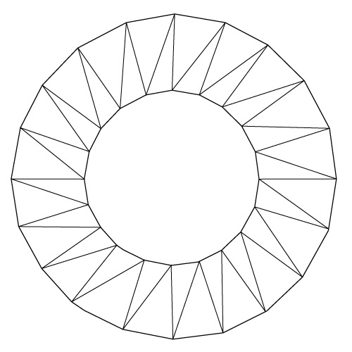
Fig. 5. Higher quality tessellation
Since the quality of the tessellation proved to be crucial for the success of the algorithm, I decided to throw away the first attempt and try a different approach which luckily ended up working much better: in Version 2, given the set of coplanar vertices, we would then perform a Constrained Delaunay Triangulation over it, generating an initial set of triangles filling both the inside of the outline and the holes. A Constrained Delaunay triangulation (CDT) is a generalization of the Delaunay triangulation that forces certain required segments into the triangulation. In our case, we need to ensure the triangulation conforms the shape by including every segment coplanar to the cut plane, with no need for a prior classification to tell whether it belongs to an outline or a hole. Fewer steps involved, and a lot more robust.
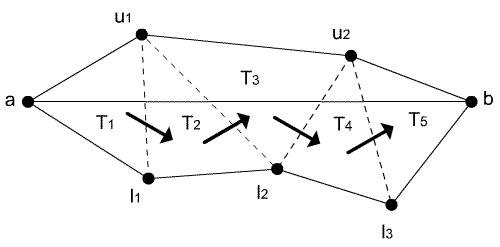
Calculating a CDT involves generating a regular DT first, and then progressively insert the required edges by removing all the intersecting triangles and re-tessellating the affected area (Figure 6). I based my implementation on [Domiter 04], which is quite nicely explained. There’s a detail that is not covered in that text, which is how to get rid of the triangles that fill the hole loops (inner circle in Fig. 5). The author proposes using a seed point provided by the user to start a triangle-killing greedy traversal on neighbor triangles. What I did instead in order to provide a (rather ineficient) automatic alternative was to start on each triangle centroid and trace a semi infinite line to count the number of intersections with each one of the source outline/hole edges (this excludes the new edges generated from the triangles) and this way determining whether the triangle is inside or outside the shape -being discarded in the later case-. You can find some explanatory diagrams in [Rupert].
This method vastly improved the quality of the tessellation, and the number of degenerate triangles that came out of further slicing it. Had it not been enough, though, I would probably had required to go one step further and implement a Conforming Delaunay Triangulation which would further reduce the distortion of the resulting triangles by splitting long edges.
Numerical Robustness
A final note about implementation details: the main issue with the method described above is that it performs many geometrc operations on a relatively small region of the mesh – A given set of faces can be sliced and reconstructed many times before the final shape of a fragment is achieved, and sooner than later this leads to problems in the form of really small, and/or almost degenerate triangles. Think of how wrong things can go when a split plane just slightly touches the geometry, or it cuts it in an odd angle leading very tiny holes which have to be filled just to be cut again on further steps.
Just like any other numeric algorithm, a good deal of care has to be put on the implementation of these operations. A big number of nasty situations can be alleviated by avoiding exact tests and using tolerances or epsilons instead. To give a simple example, when cutting out the mesh with a plane it turned out better to be slightly permissive when testing which side of the plane a vertex was on, just to avoid slicing a triangle over and over again infinitesimally away from an existing vertex. Therefore, instead of doing something like:
If (distance( Vertex, Plane ) < 0) then discard it
You would do something like:
If (distance( Vertex, Plane ) < -epsilon) then discard it
Where epsilon is a small number, so that we avoid incurring in a false positive case where a coplanar vertex decides to return a distance of -0.000001 from the plane. So far so good, but things start smelling fishy again when we find ourselves with a growing number of epsilons, magic numbers, with arbitrary small values. How should we choose them? should they all have the same value?
While it’s true that different magnitudes of “small” may suit each algorithm, and some testing will help finding sensible ranges, instead of using absolute epsilon values, it is better to make the tolerance dependent on the magnitude of the numbers you’re testing.
The reason for this is that real numbers are approximated in a computer internally by using a fixed number of bits providing a finite precision. That precision, however, is not homogeneous along the line of numbers – it converges at it’s best around 0 but then it starts degrading with larger magnitudes (Fig. 7). Taking single-precision floats, the gap between two consecutive representable numbers close to 0 is as little as 0.000001, but only 0.0625 when our numbers are in the range of millions. That’s sixty two thousand times less precise! hence it makes sense to adjust our epsilon to grow it larger with the magnitude of the inputs. If you’re interested in further details, this is all explained in better detail in Christer Ericson’s presentation for GDC ’07, and his blog and related book Real-Time Collision Detection is an invaluable reference for this and many other related topics.
The takeaway of all this is that, when comparing numbers, instead of doing:
Equal( A, B ) { return abs( A - B ) == 0; }We would then be adding a tolerance value as discussed above:
Equal( A, B, epsilon ) { return abs( A - B ) < epsilon; }
But even better, we’d make the epsilon value depend on the magnitude of our input values to make up for the non-homogeneous precision:
Equal( A, B, epsilon ) { magnitude = max( abs( A ), abs( B ) ); // you may want to clamp magnitude to 1, to avoid further // decreasing epsilon return abs( A - B ) < magnitude * epsilon; }
References
[Domiter 04] Vid Domiter. Constrained Delaunay Triangulation using Plane Subdivision.
[Rupert] Ruppert’s Delaunay Refinement Algorithm.
[Ericson 07] Christer Ericson. Numerical Robustness for Geometric Calculations. GDC 2007.
Unfortunatelly there were several problems with this approach:
First of all, identifying the closed loops from a pool of edges turned out to be harder than expected: ideally it would be a matter of finding a sequence of edges v1-v2, v2-3, v3-v4… eventually finding edge v4-v1 closing the loop. However, tiny imperfections on the mesh slicing such as parallel faces perpendicular to the plane, T-junctions, or just micro-faces which were discarded for being degenerated would cause
