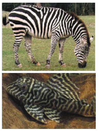
In the field of Texture Synthesis, I recently discovered the wonders of the Reaction Diffusion System for nature-like patterns synthesis. The RD method consists on a set of equations which iteratively simulate the distribution of a chemical agent (activator) modulated by the presence of another agent called inhibitor. It is believed that such interactions take place in nature to form patterns which can be found in mammals and fish, and the first model, generating spots, was proposed by Turing himself [Turing 52], dating back from 1952!.
Reaction Diffusion
 By playing with the parameters of an RD system, it is possible to simulate a variety of patterns ranging from spots to stripes. Unfortunately I haven’t found huge amounts of information on the subject (let alone up-to-date resources): one of the most complete texts is Greg Turk’s thesis [Turk 91], which covers both Turing-like spots and stripes. For the later, the most extended set of equations is the one proposed by [Meinhardt 82] which generates the kind of images I wanted to achieve.
The main problem in practice, however, is that Meinhardt’s description consists on 5 equations with several magic constants (which might make sense in chemical terms, but the authors seem to obviate) that lead to a large search space. Even more fun, the system is really sensitive to small variations on the value of each constant, and I spent quite a lot of time searching for a set of values which was stable and converged to something meaningful. Luckily, [Asai 99] and [Kondo 09] provide an alternative formulation of Meinhardt’s RD system, and an illustrated set of values to play with, which is how I ended up implementing it.

RD Strip system as appears in |Asai 99|. The reference value for the constants is a ˆ= 0.08, b =ˆ 0.08, c ˆ= 0.28, d =ˆ 0.03, e =ˆ 0.1, f =ˆ 0.15, g =ˆ 0.05
Below is an applet created with Processing which illustrates the process, it starts with a randomized concentration of the activator an inhibitor agents, and a small set of frozen points in the grid which help creating “vortices”. If you let it run long enough, it should converge to a nice seamless pattern with spirals (not that I’ve seen a fish with that pattern, but it would be cool!).
'Space' key to reset simulation. 'Enter' key to stop. Built with Processing
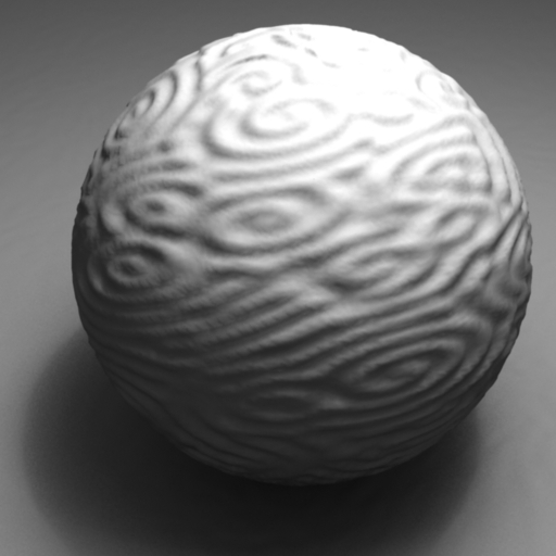
And it produces some great displacement maps!

References
[Turing 52] Turing, Alan, “The Chemical Basis of Morphogenesis,†Philosophical Transactions of the Royal Society B, Vol. 237, pp. 37–72 (August 14, 1952).
[Meinhardt 82] Meinhardt, Hans, Models of Biological Pattern Formation, Academic Press, London, 1982.
[Turk 91] Turk, Greg, “Texturing Surfaces Using Reaction-Diffusion” Ph.D. Thesis, 1981
[Asai 99] Rihito Asaia, Emiko Taguchia, Yukari Kumea, Mayumi Saitoa, Shigeru Kondoa, “Zebrafish Leopard gene as a component of the putative reaction-diffusion system”.
[Kondo 09] Shigeru Kondo, Hideaki Shirota, “Theoretical analysis of mechanisms that generate the pigmentation pattern of animals”, Division of Biological Science, Graduate School of Science, Nagoya University, Furo-cho, Chikusa-ku, Nagoya 464-8602, Japan