These are some notes on things I learned while researching the topic of watercolor simulation for a project I worked on. Due to the nature of the project I can’t provide specifics or any source code this time, but I think the basics of the problem make for an interesting topic to write about.

Image decomposition

The problem I was aiming to gain insights on is how to take a set of primary colors forming a palette, and lay them down in a set of individual images which, when later combined, would approximate the tones from a source image. This process would eventually happen on a physical medium by reproducing the layers in watercolor or a similarly translucent pigment-based medium, aiming to blend them all over paper to produce an artistically inspired rendition of the original photograph.

The process starts in the computer by scanning the pixels of a source image and decomposing them into a set of contributions for each one of the tones in a palette which is fixed and given upfront. Because we’re simulating a translucent media, this decomposition also has to have a notion of opacity associated to the pigments, which turned out a bit more involved as we’ll elaborate on below. The decomposition process has to work out in such a way that once we stack the resulting color layers together, the resulting blended colors approximately match the original reference.

Framing the problem

When I set off to tackle simulating the blending of colors I did some Googling which came up with a fair amount of interesting papers on “holistic” approaches to paint simulation which include the interaction of medium and the pigments, as well as the fluid motion of the pigments and even the brush. For great examples of these systems check out [Watercolor] and the very recent [Wetbrush] which has some really impressive videos showcasing their painting system.
These methods however sounded a bit overkill since I was mostly interested on the part about pigment blending and not so much in simulating the fluid, given that the actual painting process would happen physically. Even though my first attempt was some simple CMYK color space with with multiplicative layer blending, this ended up not being enough as I’ll describe below, to capture the range of behaviors of paint. Thus I ended up acknowledging that some of the complexity was justified, and going for a more physically-based take on the interaction between water and medium.

Solution space

Thinking of colors as vector in a 3-dimensional space -we’re sticking to tri-stimulus and putting aside more advanced spectral rendering for the time being- a target color can be expressed as the combination of a set of basis vectors constituted by our choice of palette. We’ll note a couple of implicit assumptions made here already: first that the color response is linear -and we know this is often not the case– and also that the contributions for each of the color basis will be between 0 and 1; that is, we can’t add an infinite amount of color, nor we can add a negative amount. Depending on the choice of basis, especially if the vectors are not orthogonal or there are many linearly-dependent vectors, there might be target tones that are simply not reachable by adding vectors with positive coefficients, or perhaps at all. For instance if our color basis is made up of red, yellows and oranges, no matter how many of them we add, we’ll not be able to generate green hues as they’d require a negative amount of red. Similarly there is no combination of these tones which yields to blue because we simply have no blue components.

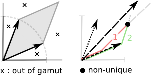
In fact for this particular application will be tackling the vector composition from the opposite angle: from a given color in the photograph describing a point in our sample space, what is the set of weight coefficients on each of the basis vectors which yield to it (these would be the paths in red and green in the illustration above). This can be expressed as:

$\vec{P} = w_0 \vec{B_0} + w_1\vec{B_1} + w_2 \vec{B_2} + .... + w_n \vec{B_n}$

or more succinctly in matrix form as:

$B*\vec{W} = \vec{P}$

From this a range of solutions might arise: in an ideal case our palette would be a beautiful orthonormal basis which would simply let us dot-product the result which each one of the vectors to obtain the corresponding weight coefficient. More likely however, most of the basis vectors will be linearly dependent, and if a solution would exist, it would probably be non-unique and a set tone could be obtained via more than one possible combination of source colors. At this point the problem becomes more of an optimization process, perhaps along the lines of “for a given destination color, what’s the combination of weights which minimizes the amount of paint”, although in this case it is not clear what the fitness function should be. Furthermore, we have yet to consider the additional degree of freedom which is the layer opacity, which adds an extra dimension to the problem.

So I wanted to constrain the problem in order to simplify it into something more defined. The first observation was that since the intention was to print the layers in a physical medium, it made little sense that each pixel on the layer image would have a potentially unique opacity. It is more reasonable to assume that the transparency of a layer is fixed and constant across its surface, and thus we can consider this opacity a property of the medium and not the pigment. The second observation is that because layers are stacked, there’s just a finite number of combinations for each individual color, namely the number of unique combinations for the layers in a particular order. This number happens to be manageable for a small number of layers, which would be in the order of 10. Under these conditions, a simple algorithm can be written as:

Given a set of colors in an input palette, combine them in all valid possible combinations and generate a set of swatches for each possible combination of layers, storing what set of weights led to it. For each pixel in the reference image, we measure the distance to each swatch sample, and pick the closest candidate. Next write out the pixel location on each one of the constituent layers of the color swatch.

This is a much simpler brute-force algorithm. Note how the number of pre-mixed swatches (i.e. the possible range of colors) grows steadily with each new addition to the palette, but even so, the processing times are well within the reach of any computer.

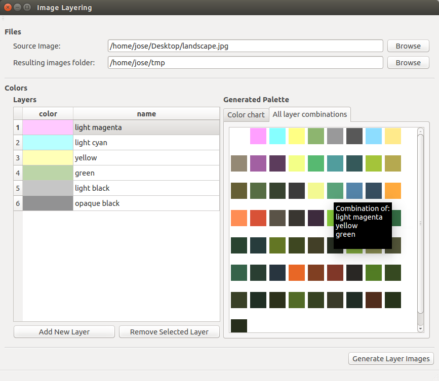
Example from an early prototype showing how the palette colors are combined to form all possible color swatches

As it turns out, I learned that painters sometimes do sometimes carry out a simplified version of the proposed swatch combination in order to get familiar with the behavior of their pigments. They do so by generating images like the one below, where each color is overlaid with each other in rows and columns. This image shows the interaction of each pair of colors in a given available range, but it also shows that the order of composition matters; note how symmetrical entries in this matrix are not entirely equivalent: while in translucent tones the order is not very important, more opaque paints tend not to mix that much and thus the top coating predominates.

On the left, a real color chart. Center and right images are reproductions of different kinds of pigments. Images from [RealPigment]

With the above approach we no longer need to worry about decomposing color combinations into its constituent pigments, but instead do so by comparing final results directly. We still need a good approximation of this blending process which mimics what will happen in reality once the resulting layers are stacked, which is what will give us good rendering of the pre-mixed color swatches we’re comparing against. This is what we’ll discuss next.

Blending colors

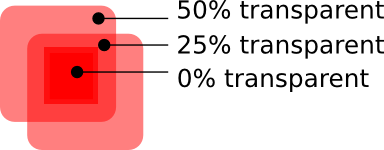Eventually we will want to produce a method that stacks a given number of input colors layers in a known order, but before going to a fully-fledged solution let’s first analyze the simplest possible situation, involving only an opaque substrate and a translucent color layer on top of it. As mentioned above, this being printed medium, the very first thing I attempted was to model a subtractive blending model by using both color multiplication or subtraction, but this wasn’t enough to capture the right appearance; multiplication is problematic because it doesn’t accumulate in an intuitive way for the painter: layering two coats of 50% transparency would yield to a 25% transparent result, instead of the expected 0%. Layer subtraction on the other hand fixes this, but we can’t model opaque pigments this way either.

The model we use has to capture a series of light scattering events happening in real life. Our target medium is made up of a pigment-based paint dissolved in a given amount of carrier -e.g. water- which lets a portion of the light pass through it to the next layer, while possibly absorbing and/or scattering some of the energy . A given ray of light passing through a layer might hit a particle of pigment with some probability proportional to the layer opacity, or simply pass through the medium. For the sake of simplicity we’ll ignore any light bending due to refractive properties of the medium because layers are assumed to be extremely thin, and assume that if no particle is hit, the light beam simply continues along unperturbed. Upon hitting a pigment particle however, some of the light energy will be absorbed, and the light colored according to the remaining wavelengths; next, the light ray can either be transmitted along the same direction, or scattered in some other direction. This set of interactions is repeated over and over again till the light is completely absorbed or ends up getting back to us. We consider in our model that the bottom-most substrate is a non-transmissive white layer, which reflects a portion of the incoming light back without any further coloration.

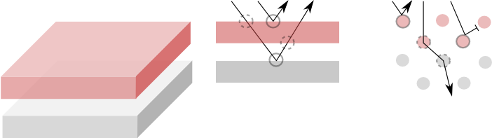
With this set of interactions we can model the paint opacity as an increase in the probability of hitting a pigment particle. Also the balance between light transmission and scattering in a hit event describes the behavior of the pigments dissolved in the carrier: watercolor can be thought of as a mostly transmissive pigment, much like colored glass, whereas something like oil paint could be considered to mostly scatter the light back to us without so much interplay with the underlying medium. Note this is all a conceptual framework loosely based on the behavior of dielectric materials which I’m using to describe the kind of interactions we’re after. Any real material is likely to be a much more complex combination of heterogeneous media and multiple light scattering, but at least this sets the basic interactions which help explain why we can’t simply get away with linear combinations of layers.

Kubelka-Munk model

Given the above observations and after some more Googling I came across the mention of the Kubelka-Munk model for color [Kubelka] mentioned in some papers. Dating no less than of 1931, the KM model describes pigments in therms of their scattering ( $S$ ) and absorption ( $K$ ) coefficients, which are wavelength-dependent and need to be captured from real samples with a spectrometer. With these coefficients we can work out a reflectance value for the pigment as a function of the spectrum wavelength which is combined with the reflectance of underlying pigments or substrate to give us the final perceived color. The original paper is in German, but some of the translations I found are hard to parse. I have instead taken the relevant equations from the [RealPigment] and [Watercolor] papers which are more concise.

Assuming we have the measured scattering and absorption coefficients, and given a thickness value for the layer we’re trying to model:

(1) $\begin{align*}R&=\frac{1-\epsilon(a-b\coth bSh )}{a-\epsilon+b\coth bSh }\\ a &=1+\frac{K}{S}\\ b &= \sqrt{a^2-1} \end{align*}$

where $h$ is the thickness of the pigment layer, $S$ and $K$ are the pigmentâ€™s scattering and absorption coefficients, $\epsilon$ is the substrate reflectance, and $R$ is the resulting reflectance of the pigment layer which is what we’re after. Note those are parabolic sine and cosine. The above is taken from [RealPigment] and all of these quantities are per-wavelength, so a pigment $\vec{p}$ is modeled as a set of scattering and absorption coefficients over a set of wavelengths L, $\vec{p} = \big\{(S_i, K_i)\big\} \forall_{i \in L}$ .

Interestingly there is an alternative formulation in [Watercolor] which expresses the same reflectance value $R$ , as well as transmittance $T$ , as follows:

(2) $\begin{align*} R&=\sinh \frac{bSx}{c}\\ T&=\frac{b}{c} \end{align*}$

where,

(3) $\begin{align*}c=a\sinh bSh + b \cosh bSh\]\end{align*}$

The $a$ and $b$ variables are the same as above, and $h$ is again the layer thickness. These two formulations are equivalent as one would expect, and I have added some additional notes at the end of this article on this regard.

It is $R$ and $T$ that we’re eventually interested in, since those are the properties of the layers which will allow us to compute the final reflectance corresponding to the visible color getting back to us. When we have multiple stacked layers, we can compute the reflectance and transmittance by recursively applying:

(4) $\begin{align*} R&=R_1 + \frac{{T_1}^2R_2}{1-R_1R_2}\\ T &= \frac{T_1T_2}{1-R_1R_2} \end{align*}$

Where $R_1$ and $T_1$ correspond to the reflectance and transmittance of the coating layer, and $R_2$ , $T_2$ to those of the substrate layer. The reflectance we’ll use for the final color of each swatch we compare against is the result of combining $R$ and $T$ as light travels through all the layers that make up such swatch.

Heuristics for computing the S and K coefficients

Because we don’t want to rely on a spectrometer to measure the scattering and absorption coefficients for pigments (though some of those values are known for common pigments), we need to provide a method to obtain the coefficients from RGB colors an artist can choose from. There’s a variety of heuristics proposed for this, and the general problem is that a single RGB value is usually not enough information to reconstruct $S$ and $K$ , as we need to incorporate knowledge on how the pigment scatters, how it absorbs, and also the layer thickness $h$ . The RGB value we obtain from a color picker in a computer only gives us information about the reflectance of that particular color.

Various synthetic pigments generated using the Kubelka Munk theory and the heuristic proposed in [Watercolor]

I ended up implementing the heuristic described in the [Watercolor] paper, where they obtain the $S$ and $K$ coefficients from two reflectance samples, namely: $R_w$ or reflectance on white, which can be read as ‘what does the pigment look like over a white background‘ and $R_b$ , reflectance on black, or ‘what does the pigment look like when laid over a black background’. $R_w$ gives us information about the reflectance of the pigment, whereas $R_b$ gives us information about the transmittance – the thicker the pigment is, the less black we’ll see through it. There is a restriction in the possible values we can choose from, which must satisfy $0 < R_b < R_w < 1$ The authors of the paper generate some beautiful charts to illustrate the method; in the color swatches of the illustration above we can see the effect of varying the layer thickness as well as the reflectance of each pigments over a white and black background. Note the difference in opacity between (b) and (h), as well as the subtle shift in hue in the later.

From the two reflectance values we obtain the scattering and absorption coefficient as:

(5) $\begin{align*} S&=\frac{1}{b}\coth^{-1}\bigg(\frac{b^2-(a-R_w)(a-1)}{b(1-R_w)}\bigg)\\ K&=S(a-1) \end{align*}$

Where $a$ and $b$ are rewritten as:

(6) $\begin{align*} a&=\frac{1}{2}\bigg(R_w + \frac{R_b-R_w+1}{R_b}\bigg)\\ b&=\sqrt{a^2-1} \end{align*}$

Note all these quantities are always per wavelength, which in our case it will bean they’ll be computed independently for the red, green and blue channels.

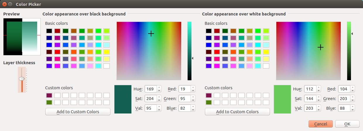
Thus, for any given pigment we want to incorporate in our palette we need to specify two RGB colors: reflectance on white and reflectance on black, as well as the desired thickness for the associated layer. Because this is a lot to ask from the user, I ended up implementing a -rather intimidating- color picker similar to the one described in the paper, which runs the equations to display a preview image with the pigment laid over both a white and black background, and a varying degree of thickness running vertically. It is subtle, but notice how it is possible to obtain different hues from the same pigment by tweaking the different values.

The above formulation represents just one possible heuristic I found easy to reason about. The [Ukiyoe] paper takes this idea even further and provides a heuristic requiring only one color by imposing however further assumptions on the medium. Eventually I found it a bit restrictive for my intended usage and ended up going back to two-reflectances method, but it might be interesting to go back to it in the future and analyze the differences.

The final process

Putting it all together, our final workflow is as follows:

Generate a set of input palette colors specified via their corresponding $R_w$ and $R_b$ RGB values, as well as a layer thickness $h$ for each one of them.
From the above values we work out the scattering $S$ and absorption $K$ coefficients for each palette pigment (Eq. 5, 6).
Produce all the pre-combined color swatches by obtaining the reflectance $R$ and transmittance $T$ coefficients for each pigment (Eq. 1,2,3), and combine the pertinent layers by recursively applying (Eq. 4).
brute-force search the closest match amongst the color swatches to each of the target image pixels, comparing the distance between their reflectance values. Note here we can take any metric, and opt for any alternative color space such as HSV.
For each of the constituent layers of the chosen swatch, set the corresponding pixel position signaling the layer does contribute to the active pixel. This and the above step can be trivially parallelized per pixel.
In order to produce a preview of what the image reconstruction will look like we can simply replace each source pixel by its closest swatch color (since these are already pre-mixed) or we can alternatively carry out the reconstruction at a later stage from the $S$ and $K$ coefficients of each of the layers contributing to any given pixel, combined using the aforementioned equations.

Because the layer blending mode is quite involved, it is not possible to do a rough approximation of the final image in Photoshop with any of the standard blending modes. Instead the image was being approximated as the decomposition took place in the application. Unfortunately I don’t have any of the physical prints available to do a direct comparison with the KM model, but I’ve attached one of the test images produced while prototyping the system. It is very evident that the decomposition as it currently stated would generate very speckled layers, with lots of high frequencies. When trying to reproduce these by hand it is to be expected that the contours would be greatly smoothed out, which would make their overlap inaccurate around the edges, possibly adding some interesting hue shifts around these areas.

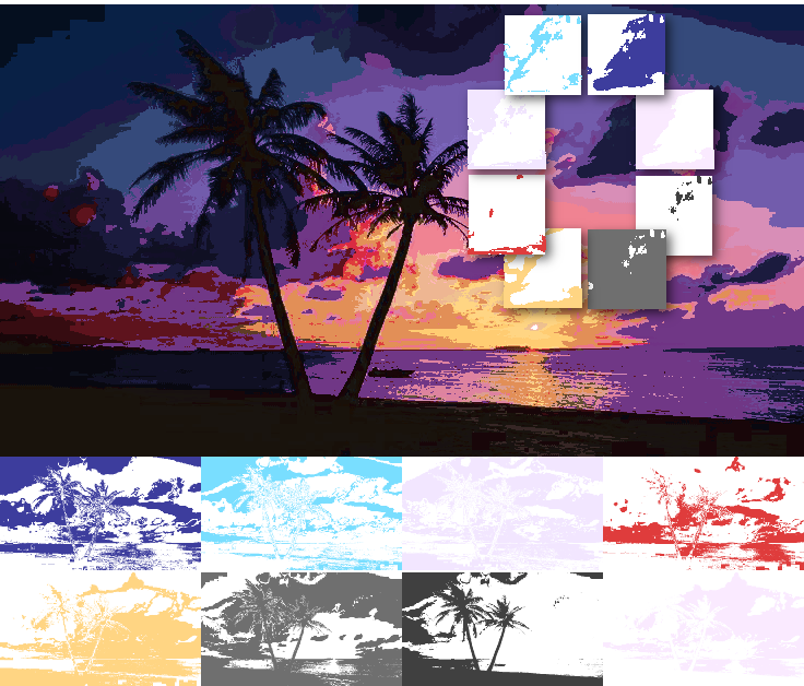
Composition preview given a number of layers shown below. The circled area on the left shows a detail closeup, note how none of the input layers adds a purple tone directly, but the tone is obtained from the combination of overlapping layers.

Composition preview given 8 palette colors shown below. The circled area on the left shows a detail close-up, note how none of the input layers adds a purple tone directly, but the tone is obtained from the combination of overlapping layers applying the KM equations.Â Note at this stage the image is still essentially a glorified color decimation process, and needs of the artist interpretation in order to become a proper watercolor.

Additional notes

Since I’ve been putting together the various equations from a couple of sources, we now have a couple of seemingly equivalent ways for obtaining the reflectance of a coating layer over a substrate from the input scattering and absorption coefficients and layer thickness. That is, given $S$ , $K$ and $h$ , and assuming a perfectly reflective substrate, we can:

Option 1. Apply the KM model as described in [RealPigment] and [Ukiyoe] (Eq. 1):

$\begin{align*} R &= \frac{1-\epsilon(a-b\coth bSh)}{a-\epsilon+b\coth bSh}\\ a &= 1 + \frac{K}{S}\\ b &= \sqrt{a^2-1} \end{align*}$

Option 2. Proceed as described in [Watercolor] by obtaining $R$ and $T$ from the scattering coefficient (Eq. 2, 3), then applying Eq. 4 for compositing on top of the white substrate to obtain the final reflectance:

$\begin{align*} R_1 &= \frac{\sinh bSh}{c}\\ T_1 &= \frac{b}{c}\\ a &= 1 + \frac{K}{S}\\ b &= \sqrt{a^2-1}\\ c &= a\sinh bSh + b\cosh bSh \end{align*}$

Then composite with Eq. 4. We can model the same substrate as above by setting its reflectance to $R_2 = \epsilon$ and the transmittance $T_2 = 0$ but this imposes no loss of generality in the validation we want to carry out:

$\begin{align*} R &= R_1 + \frac{{T_1}^2 R_2}{1-R_1 R_2} = R_1 + \frac{{T_1}^2\epsilon}{1-R_1\epsilon} \\ T &= \frac{T_1 T_2}{1-R_1 R_2} \end{align*}$

And we can summarize the check as:

$\frac{1-\epsilon(a-b\coth bSh)}{a-\epsilon+b\coth bSh} \stackrel{?}{=} R_1 \frac{\sinh bSh}{c}+ \frac{{T_1}^2\epsilon}{1-R_1\epsilon}$

Which can be written in terms of $a$ , $b$ , $S$ and $h$ by performing the necessary expansions. This turns into some hairy terms especially since we have a $R_1$ term in the denominator; I did some attempts by hand without much success and then I ended up feeding the above equations to Mathematica which pretty much confirmed the equality, but in a rather opaque way (the breakdown is here). Not convinced, I ended up carrying out the check numerically by writing a short Python program which calculates reflectance for a range of values of the aforementioned input variables and indeed, it all seems to check out. If anyone reading this can find a cleaner way of proving the equality, I’d love to hear about it.

References

[Kubelka] Kubelka and Munk. The Kubelka-Munk Theory of Reflectance. Zeit. FÃ¼r Tekn. Physik, 12, p593 (1931).

[RealPigment] Jingwan Lu et al. RealPigment: Paint Compositing by Example. NPAR 2014, Proceedings of the 12th International Symposium on Non-photorealistic Animation and Rendering, June 2014

[Watercolor] Curtis, Cassidy J., et al. Computer-generated watercolor. Proceedings of the 24th annual conference on Computer graphics and interactive techniques. ACM Press/Addison-Wesley Publishing Co., 1997.

[Ukiyoe] Hirokawa, Tomotaka, et al. “Generating Digital Image of Ukiyoe by Applying the Kubelka-Munk Theory.” NIP & Digital Fabrication Conference. Vol. 2005. No. 2. Society for Imaging Science and Technology, 2005.

[Wetbrush] Zhili Chen, Byungmoon Kim, Daichi Ito and Huamin Wang. 2015. Wetbrush: GPU-based 3D painting simulation at the bristle level. ACM Transactions on Graphics (SIGGRAPH Asia), vol. 34, no. 6.

Aiding watercolor paintings