It’s been a while since the last post, and the truth is I’ve spent most of my spare time lately devoted to my photography. Back however to more technical matters, one of the topics I find fascinating is NPR techniques, and particularly Stippling as an interesting example of them. I’ve been reading about it for some time now and learnt a couple of interesting things along the way, so I thought I would share them in a post.
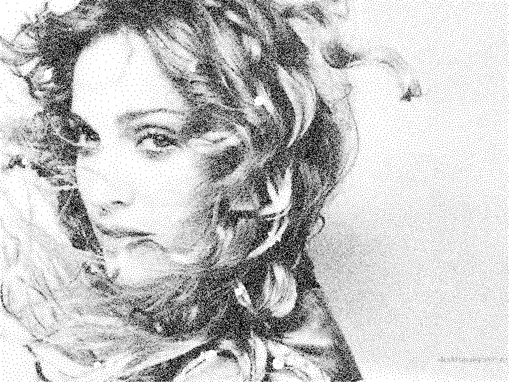
When stippling an image, we’re basically interested in generating a distribution of points with a density distribution matching the tones of the original image, the size of the points is generally constant, and we add more or less of them to create darker or lighter tones. In these areas it is important to generate a distribution free of sampling artefacts, which manifest as patterns in the image — the eye is really good at picking up these.
So essentially all we need is a big number of points distributed randomly, and a way of quantizing their required density when we place them over the image. To generate the points, the first approach would be using purely random points. It turns out, however, that pure randomness does not lead to aesthetically pleasing results, as points tend to clutter in areas and leave empty spaces. On the other extreme, using a perfectly homogeneous scheme — say a grid- would lead to artefacts in the form of aliasing. We thus need something still random but still somewhat a bit more even.
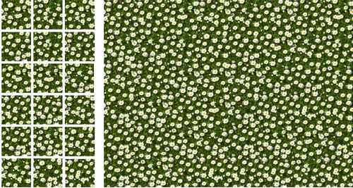
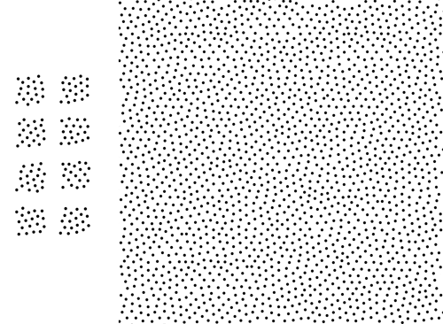
In the in-between land, there’s a flavour of noise called Blue Noise, which is the name given to a particular distribution of frequencies with minimal low-frequency components and no concentrated spikes in energy. This means that we have no structural aliasing given by the low frequencies, and even spacing with minimal cluttering. It is generally accepted that blue noise properties make for some of the best sampling patterns for a wide range of applications (see [Lopez 10]).
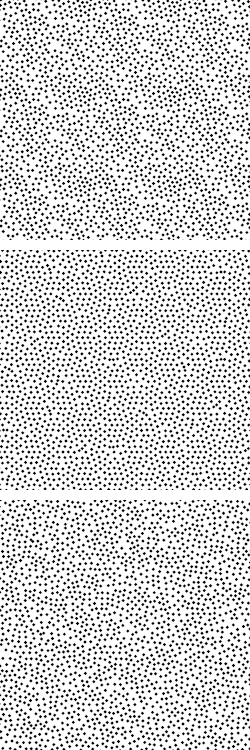
Noise patterns: the top image shows structural repetition. The middle one displays radial patterns and clustering. The third one displays blue noise characteristics. Images from |Kopf 06|
One way of generating point distributions with blue noise properties is by means of a Poisson-Disk Distribution [Cook 86]. One of the most straightforward ways of generating such distribution is by using a so-called Dart-Throwing Algorithm [Cook 86], which generates candidate points in a random fashion over the plane, but will only accept each candidate if it lies at a minimum distance from every previously accepted sample. McCool and Fiume [McCool 82] describe a more practical variant
of dart throwing, where the dart radius gradually decreases as more samples are placed. The Dart-Throwing algorithm is therefore inherently sequential and slow due to its quadratic complexity, but the quality of the results is nevertheless high.
An important property of any distributions generated with the aforementioned variation proposed by McCool and Fiume is its progressiveness: Similarly to some low-discrepancy sequences, if we put all the generated points into a list of N elements, and draw only a portion of that list [1, N < M], the resulting point distribution also covers the entire plane (as opposed to sweeping it), but simply does it with a lower density. This is important because it means that if we can stipple a spatial region with a given density by plotting all the points of a tile T, we will also be able to generate any lighter density by using the same T by plotting a smaller set of its points.
The amount of points we typically need to stipple an image, which is in the range of thousands in the best of cases, makes the straightforward implementation of the dart-throwing algorithm impracticable. A big part of the problem we’re facing with stippling is how to efficiently generate lots of points in a blue noise distribution. There is a significant amount of research on the matter, and the rest of the post will deal with a couple of approaches I liked and implemented myself, along with notes on related work.
Efficient generation of Poisson-Disk Point Distributions
To generate PD point distributions with blue noise properties there are several families of approaches, among which we have:
- Incremental methods, which place samples sequentially. The Dart-Throwing algorithm described above is a basic example of them, but one could easily come up with more sophisticated implementations which made use of auxiliary structures such as hashing grids or trees to reduce the cost of the nearest-neighbour lookups. A proposal I found particularly interesting is described in the paper [Lopez 10], further details on the implementation of this method are provided below.
- High-throughput methods: these usually rely on a heavy precomputation stage but a very fast execution time. A prime example of this kind of algorithm is [Kopf 06], also implemented and described in this post. Also, impressive results are obtained by [Wei 08] with a GPU-based Poisson-Disk distribution generation algorithm, orders of magnitude faster than the sequential approach.
- Approaches based on Constrained Voronoi Diagrams (CVD), where each sample corresponds to a cell. These approaches, despite being extremely expensive in time, generate probably the most pleasing distributions. [Hongwei 09] report gains of 10x in execution time in their paper.
The differences between types of approaches are quality (depicted as even, perceptually pleasing distributions) and execution time. The best results seem to be obtained with CVDs or sequential algorithms, but their execution times are orders of magnitude slower than high-throughput approaches such as the one based in Wang Tiles, which run in real time. These later generate a more noisy result however, which as we’ll see, may not be so much aesthetically pleasing for the particular case of stippling – Nevertheless blue noise sampling may be used for a variety of applications such as object- or texture-placement as the authors show in the [Cohen 03], where the density of the distribution will likely be much less dense and speed is crucial.
Adaptive Incremental Sampling
The first one of the approaches I tried is the one described in the paper [Lopez 10], which is a more efficient extension of a sequential algorithm with good quality results and decent execution time.
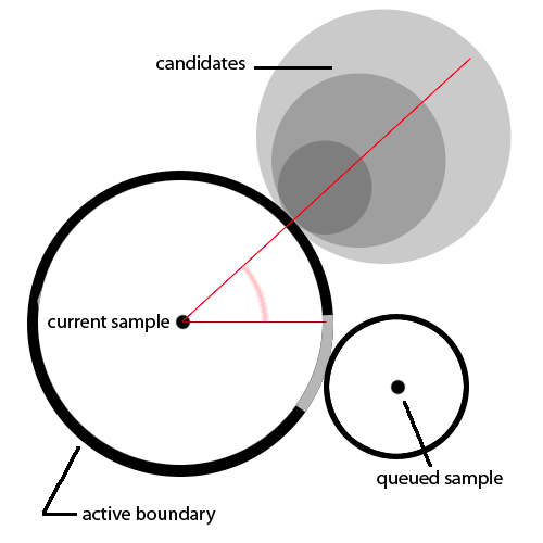
The key idea behind the approach is simple: having a sample point on the plane, and a minimum acceptance distance limiting how close any other sample can get to it, we build a disk and generate all subsequent samples on its boundary*, instead of randomly on the plane. For each accepted new sample, we calculate the intersection between its disk and the currently active one and subtract a portion of the active boundary area — so no new samples will overlap. When there’s no remaining boundary on the active disk, we de-queue it and proceed with the next one.
This defines a pattern in how the samples are generated, as new samples are only generated on the currently active disk, and their corresponding disks are queued for later processing. The samples then grow across the image from an initial seed (which it’s quite pretty to watch!). A secondary image buffer is kept to speed up disk overlapping checks, where disks are rasterized. In order to accept a sample we have to first check whether the corresponding rasterized disk would overlap a non-empty pixel in the disk buffer.
The acceptance distance for any sample is given by the density distribution, i.e. the amount of black, in the region covered by the sample on the source image
* More precisely, an angle is sampled on the remaining boundary of the active disk. The new disk will be placed on the line that parts from the centre along the direction defined by this angle, at a distance given by the image densities of both the active and the new disk.
Implementation notes
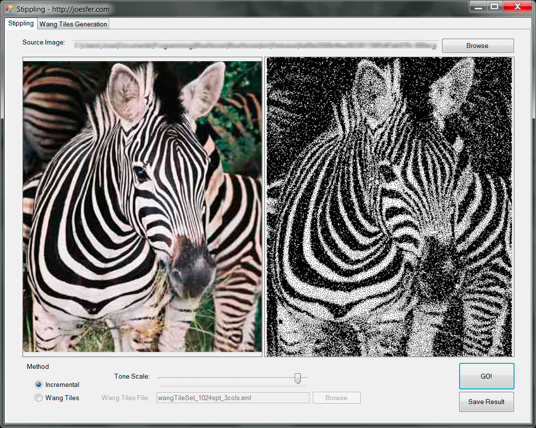
As part of the test application provided at the end of this post, I worked on an implementation of the AIS algorithm using C#. Despite the running times I’m achieving are not nearly as fast as the ones reported in the paper, they’re not too bad for the quality. Although this is conveniently omitted in the paper, care has to be taken when implementing the disk adjustment heuristic to deal with sub-pixel disks, especially as they tend to make the process diverge, and may even get the algorithm stuck due to the inability of the disk image buffer to handle disks smaller than 1 pixel. I found using a correct disk area calculation (as opposed to a squared window approximation) to produce fewer artefacts albeit slightly slower. Dark images such as the zebra displayed in the screenshot below are remarkably difficult to handle robustly due to the high contrast and sample densities required
This being said, the results look pretty nice in most cases. There’s a free parameter which controls the overall density of the stippled image — not every image is suited for a fixed value of this parameter, and tinkering with it helps achieve optimal results.
Recursive Wang-Tiles
The second approach I tried belongs to the high-throughput family described above. This algorithm relies on a heavy precomputation stage to generate an auxiliary structure called Wang Tiles used in combination with PD distributions to achieve fast running times.
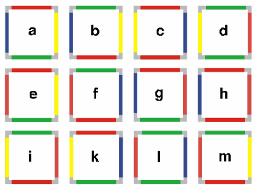
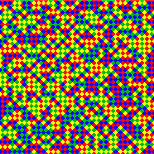
Wang Tiles [Cohen 03] are a construction which enables arranging a finite set of elements (the tiles) in a non-periodic (pseudorandom) sequence to cover the plane. The tiles are squares which have a colour assigned to each one of its four edges. The algorithm states that a tile can only be placed if the colour of its edges matches those of the surrounding tiles that have been previously placed. For any set of tiles whose elements fulfil the required restrictions, an element is chosen randomly.
We start with a tile and sequentially insert random tiles from left to right, simply ensuring that the left edge colour on each newly placed tile matches the right edge colour of the last one. Once we’ve reached the right bound of the area to cover, we continue building a new row, now matching the left and top edges with the tiles from the previous row. This is called the scanline algorithm.
We start with a fixed set of tiles and place them satisfying 1 or 2 restrictions depending on how many neighbour edges we need to match at any given time. For C possible edge colours, we’ll need at least N*C2, N>=1 tiles available to satisfy every restriction on the top and left edges. N determines the number of available choices for any placement, from where we chose using a uniformly distributed random number.
What it’s interesting about the sequence generated by the aforementioned algorithm is its aperiodicity, its lack of structure or repetitive patterns.
Now, what do we put in the tiles? Wang Tiles have been used to synthesize textures from samples; we’ll use them to cover the plane with a noise pattern, generated from a finite, relatively small, set of PD distributions. This process is described in the paper [Kopf 06]. Having this, all we need to do at runtime is execute the scanline algorithm to cover the desired image area with tiles from the pre-computed set.
Before that, there are a couple more details to worry about: edge seams and recursiveness.
Edge Seams
By simply choosing random squared samples of textures or noise patterns and then putting those together next to each, we won’t guarantee that the seams match. We need to build the tiles in such a way that, whenever the edge colours on the opposite edges match, so does the image on the tile.
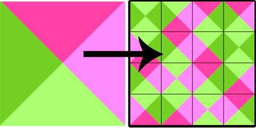
To do this, the authors propose choosing square samples for the colours themselves, and then combining those sample colours to build each tile (4 source images for each tile) as depicted in the figure below:
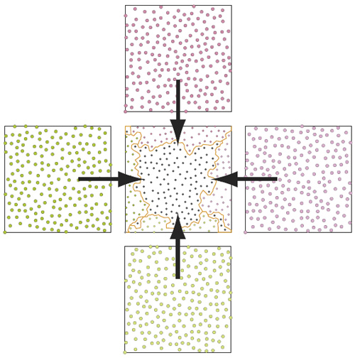
Tile merging: a source distribution is generated for each tile, and then merged with 4 additional distributions corresponding to each edge colour. This will ensure the contents of adjacent tiles match the boundaries. Image from |Kopf 06|
This way, since each matching edge comes from the same image, they will align properly.
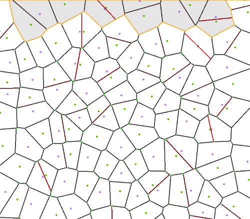
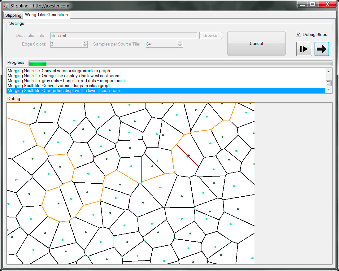
For the case of blue noise samples however, things get a bit more involved: we not only need the noise patterns to match on the edges, but we also need the resulting merged tiles to preserve their PD properties: we don’t want merged samples to form clusters. The authors of [Kopf 06] propose making use of a Voronoi diagram containing all the samples to be merged and then building a seam from the path that minimizes a cost function which penalizes nearby samples. Put in plain words, this means merging the source PD distributions by cutting along an irregular seam passing by those areas where points are further away on average.
After this stage, we’ll have a set of tiles that we can blindly arrange according to the scanline algorithm to generate a sequence which will also preserve PD distribution properties. Note that generating the Wang Tiles is the bulk of the work in this algorithm, but it’s a one-off process. After that, we’ll be able to cover as much area as we want with blue noise without having to run a sequential dart-throwing algorithm at runtime.
Recursiveness
The second issue we have to worry about is: we know our source tiles are progressive, and therefore plotting a subset of them produces a less dense, but equally filling noise distribution. We use this property to generate light shades on our stippled image – but if we happen to require more density than the maximum our tiles’ distribution can provide, we won’t have enough points!
We thus need to make the tiles recursive: allowing any tile to be subdivided into a set of NxN smaller tiles (built following the same edge-matching rules) which adds up to N2 more points than the source tile.
Recursiveness along with Progressiveness are the properties that will allow us to achieve arbitrarily dark or light shades in the stippled image.
Putting it all together
The stippling algorithm based on Recursive Wang Tiles is based on the following steps:
Preprocessing:
- Let C be the number of edge colors, generate a complete set of N*C2 source PD point distributions.
- Generate C more PD distributions, one for each edge
- Build the complete set of unique N*C2 Wang Tiles by merging each source distribution with the 4 edge distributions. Note that the original source distribution won’t match on the seams, but these merged ones will.
At runtime: Cover the source image with a non-periodic sequence of the pre-generated tiles; for each tile, decide whether to insert each point based on the required image density. If we’ve inserted all the points on a tile distribution and we still require more density, subdivide the tile.
Note that the image generated with this method is somewhat noisier than the result achieved with AIS, however, if you run the provided software you’ll notice how much faster this method is (excluding the preprocessing, that is).
Colour?
To finish the post, I wanted to provide a hint of what I consider a failed test either as a note to self or in case anybody reading this is willing to come up with an idea to make it work in the future 🙂
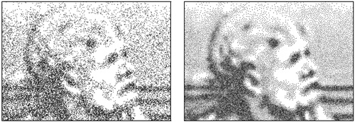
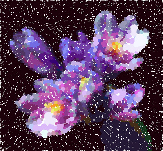
Despite personally finding the monochrome stippled images to be beautiful, one trivial extension I thought of was extending the AIS algorithm to plot coloured disks by averaging the underlying image pixels. I was aiming for a somewhat pointillist effect. However, the image doesn’t completely make it for me because the approach is basing the stipples (the strokes in this colour version) exclusively on the darkness of the image, completely ignoring the homogeneity of the tone — this will prevent dark broad strokes from appearing on the result no matter what. Obviously, that’s what the stippling algorithm is designed to do: generate dark shades from dense clustering of points, but I do think something like this could be achieved:
Downloads
An application implementing the Adaptive Incremental Sampling and Recursive Wang Tiles algorithms described in this post are provided. The source code is written in C# under Visual Studio 2010. If you just want to run it, there are binaries already built, along with a pre-generated set of Wang Tiles to use included in the compressed file.
Precompiled binaries: stippling.zip
Source code repository on GitHub: https://github.com/joesfer/Stippling
References
[Cook 86] Cook, R. L. 1986. Stochastic sampling in computer graphics. ACM Transactions on Graphics 5, 1, 51–72.
[McCool 82] McCool, M., and Fiume, E. 1992. Hierarchical Poisson disk sampling distributions. In Proc. Graphics interface ’92, 94-105.
[Kopf 06] Johannes Kopf and Daniel Cohen-Or and Oliver Deussen and Dani Lischinski. Recursive Wang Tiles for Real-Time Blue Noise. ACM Transactions on Graphics (Proceedings of SIGGRAPH 2006).
[Hongwei 09] Hongwei Li, Diego Nehab, Li-Yi Wei, Pedro Sander, and Chi-Wing Fu. Fast Capacity Constrained Voronoi Tessellation.
[Cohen 03] Michael F Cohen, Jonathan Shade, Stefan Hiller, Oliver Deussen. Wang Tiles for Image and Texture Generation. ACM Transactions on Graphics 22 (3) p. 287.
[Lopez 10] Ignacio Ascencio-Lopez and Oscar Meruvia-Pastor and Hugo Hidalgo-Silva. Adaptive Incremental Stippling using the Poisson-Disk Distribution. Journal of graphics, GPU, and game tools.
[Wei 08] Li-Yi Wei. Parallel Poisson Disk Sampling, in SIGGRAPH 2008, Association for Computing Machinery, Inc., March 2008

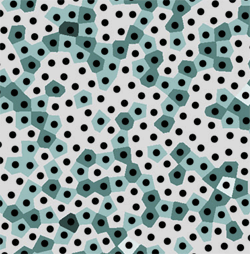

Thanks for the article and the video, it was very helpful! Another solution came up a couple of years ago which might be also very interesting:
Mohamed S. Ebeida,Scott A. Mitchell,Anjul Patney,Andrew A. Davidson,and John D. Owens. 2012. A Simple Algorithm for Maximal Poisson-Disk Sampling in High Dimensions
Thanks for the nice article. Is there a possibility to save the coordinates of the generated points rather than an image? It would be very useful for further analysis. Thanks.
No, not on the program attached on this article. The color version however does produce an output xml with the points you could parse.
i researched a stippling algorithm for myself a while ago and i choosed this one : https://github.com/MarcSpicker/LindeBuzoGrayStippling
i thought the result were beautiful and it’s relatively easy to have temporal coherence over frames.
as for the color , i naively separated each channel (rgb) and stippled them separately.you can see some results here : https://www.youtube.com/watch?v=93dm7nw29KY
thank you for the article.i learned a lot of things.
Thank you for sharing, great results!
Do you think it will be anyhow possible to export the result as an svg to be able to plot the output?
Very nice tool, congrats!!
This is something I didn’t get time to implement back when I created the tool. The software does, however, generate a text file with all the data. It should be relatively simple to write a script to convert that data into a SVG file.